Chapter7 Homework Activities
7.1 General instructions
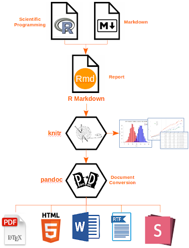
In the first week session, we talked about why we need to conduct research in reproducible manner. It facilitates transparency in research process, increases public re-usability of scientific evidence, and promotes scientific collaboration.Rmarkdown documents are reproducible and supports various output formats such as pdf, html, and docx. Rmarkdown is simply combine your R codes, documents your data analysis into a reproducible document and format.

For all activities you are expected to produce html files with the discussed answers and the relevant code. You need to generate a Rmarkdown document and use knitr to generate the html file with your answer. Create one html file for each weekly submission. This video explains how to do this. The video uses an earlier version of Rmarkdown, so you will notice that when you create a new markdown file instead a dialogue box open (select html) but everything else pretty much remains the same. In any case, you can find further details about Rmarkdown here or in this very detailed tutorial. This guide, produced for a different course unit, helps you to test drive and troubleshoot common problems. Although it may take you a while to get used to produce your homework in this way, in the long run you will see the benefits.
You have to include all codes you use for the home works. Once you knit to a html file, you need to upload the file to TurnitIn through Blackboard before the next session (e.g., week 1 homework deadline is ‘before Week 2 lab session’)
7.2 Week 1 Homework: Basic Data Exploration and Filtering
Exercise 1
Load the classic Guerry data available from the Guerry package. Hint: see the lab note 1.13 Dataframes. We got ‘hate_crimes’ data from the ‘fivethirtyeight’ package.
- How many variables and cases does this data have? Hint:
dim() - What are the names of the variables? Hint:
names() - What does the variable
Prostitutesmeasures? Hint:help() - Produce a simple histogram of the
Crime_persvariable. Any discernible patterns? Interpret and discuss your results. Hint:Hist() - Produce summary statistics of the
Crime_persvariable byRegion. Any discernible patterns? Interpret and discuss your results. Hint: see the lab note 2.7.
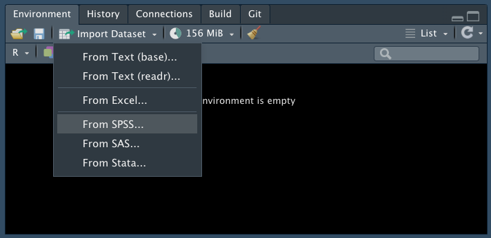
Exercise 2 Acquire the “NCVS” data from blackboard under the data for week 1. Download this into your working directory, into a data sub-folder if you have one. Import the data into R (Use ‘Import Dataset’ in the environment window. Select ‘From SPSS’.). Name the dataframe object ‘ncvs’.

- Now explore your data with some of the functions we learned in the lab today. How many observations are in the dataframe? How many variables?
- What are the possible values for the injured variable in the ncvs dataframe? What do these tell you? Hint: look for how to find labels.
- I made a frequency table for the injured variable using the code
table(ncvs$injured). I received the output names as0and1. How can I make them asuninjuredandinjured? Hint:as_factor()
Exercise 3
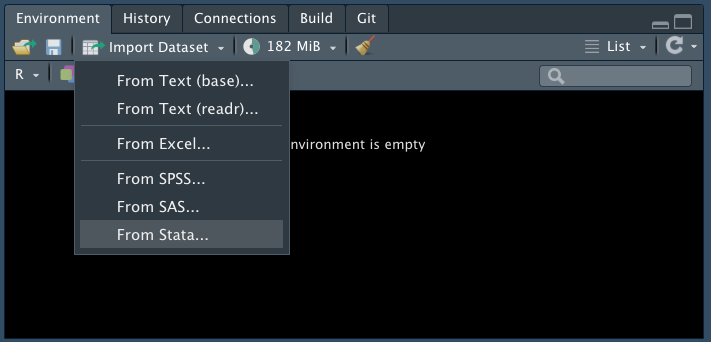
Acquire the “ukpolice” data from blackboard under the data for week 1. The data has information of ‘the number of police officer in each police force (UK)’ in 2016. You can find the relevant information here. (Use ‘Import Dataset’ in the environment window. Select ‘From Stata’. You will learn how to import data in the later weeks using R codes. Here, just try to remember R can import different types of data in various ways).

- What was the mean number of police officers in all police forces?
- Using the ‘filtering’ methods described compute the mean and standard deviation for the four largest forces and compare it with the mean and the standard deviation of the remainder police forces. Hint: see lab note 2.5. and use the ‘top4’ variable.
7.3 Week 2 Homework: Data visualisations with R
Download from the GitHub repository the following dataset crossnat.csv. You url for the dataset is: https://raw.githubusercontent.com/eonk/dar_book/main/datasets/crossnat.csv
Look at the instructions for how to download files from the web that we provided in Week 1. This comma-separated value file contains a number of variables about 194 countries. This data is collected for teaching purposes in January 2014. The information comes from a variety of sources (World Bank, United Nations, OCDE, etc) and it relates to the more recent year for which data was available then.
Sometimes students experience problems when downloading files within a Rmarkdown file. If you are getting stuck you may try an alternative. First get the file in your hard-drive using the console or a script (not Rmarkdown):
step 1 Download the file into your global environment as covered in week 1;
step 2 Save the file into your hard-drive, for example write.csv(crossnat, “crossnat.csv”) to save it as .csv in your working directory;
step 3 Then read the data from your working directory into rmarkdown (e.g., using the read.csv() function)
Ok, these are the questions:
- Display a histogram for the prison rate per 100,000 population (
prisonrate). Interpret and discuss your results. Can you identify any outliers? Are these errors? Are there plausible explanations for the extreme values in these countries?
- Produce density estimates and boxplots to compare the prison rate according to various categories of the level of human development per country (use ‘cathid’). Interpret and discuss your results.
- Produce a scatter plot with a smoothed line to examine the relationship between
prisonrateandgdppercapita. Interpret and discuss your results.
- Produce a scatterplot matrix to examine the relationship between
prisonrate,gdppercapita,urbanpop(proportion of the population that lives in urban areas) andhomicide(homicide per 100,000). Interpret and discuss your results.
7.4 Week 3 Homework: Foundations for inference (confidence intervals)
Download the following dataset Seattle_Neighborhoods_Crime_RandomSample_dar.dta from Blackbord and import the data into R. Get to know your data, specifically how many variables and observations and what the data were collected for and how the data were collected. It is always good practice to understand the data you use. For information on the methodology (including data collection procedure), see: Seattle Neighborhoods and Crime Survey, 2002-2003 (umich.edu)
There is a variable neigh_sd composing variables from variables Q14A to Q14E, which shows ‘the level of neighbourhood social disorganisation’.
- Use the
t.test()function to calculate 95% confidence interval of the mean forneigh_sd. How would you interpret the values?
- Now calculate 99% confidence intervals of the mean for
neigh_sd. How are these values different to that of the 95% confidence intervals? Why do you think that is?
Let’s look at another variable, of whether the respondent reported an incidence of theft to the police. This variable is called Q61E_f in your data. Use the attributes() function to learn about the variable. Remember this is a categorical variable so you need to transform the data into a ‘factor’ variable.
- What percentage of respondents who answered this question with Yes or No reported their theft to the police? Make sure you only keep Yes or No and remove any missing observations.
- Calculate 95% confidence intervals of the percentage of respondents who answered Yes (hint: look for the
prop.test()function in the lab notes). What does this tell you? Interpret this in your own words below.
7.5 Week 4: Hypothesis tests (comparing means)
For this task, we will use data from the Crime Survey for England and Wales. Specifically we’ll be working with data from the 2013/14 year. You can find the data on blackboard in the data for this week folder. Note the extension (.dta) so remember what you will need for importing your data.
- We want to explore the difference in fear of crime between people who have been victims of crime and those who have not. The variable which tells you how many people had been victims in the last year is ‘bcsvictim’. Re-code this variable so the values are meaningful rather than 0 and 1. (Hint: you can use
attributes()andas_factor()ormutate()andcase_when(), look through past weeks for help).
- Create a frequency table and tell me how many people in the data set were victims of crime in the last year.
- Now compare visually the distribution of the
worryxvariable between those who had and hadn’t been victims of crime in the last year. Choose the type of plot you think would be most appropriate. Who do you think has higher scores on fear of crime? Interpret this in your own words below.
- What is the mean (average) score on
worryx(fear of crime score) for those who had been victims of crime? What about those who had not?. Now what do you think who has higher scores of worry?
- Use the appropriate statistical test to tell me whether or not there is a statistically significant difference (with alpha = 0.05) in worry between those who have been victim of crime and those who have not. Explain your answer.
- What does this significant effect mean? How big is the difference in mean fear of crime scores between the groups? Explain in your own words as well this result.